Ergodic Decomposition

Posted on 20/09/2013 by Joel Moreira

— 1. Introduction —

In the study of measurable dynamics, the basic object of study is a measure preserving system: a quadruple ${(X,{\cal B},\mu, T)}$ , where ${X}$ is a set, ${{\cal B}}$ is a ${\sigma}$ -algebra over ${X}$ , ${\mu:{\cal B}\rightarrow[0,1]}$ is a probability measure on ${{\cal B}}$ and ${T:X\rightarrow X}$ is a measurable map such that, for each ${B\in{\cal B}}$ , we have ${\mu(T^{-1}B)=\mu(B)}$ , where ${T^{-1}B=\{x\in X:Tx\in B\}}$ . If there exists a set ${A\in{\cal B}}$ such that ${0<\mu(A)<1}$ and ${T^{-1}A=A}$ , then we can consider the measure preserving system ${(A,{\cal A},\nu, S)}$ , where ${{\cal A}=\{B\in{\cal B}:B\subset A\}}$ , ${\nu=\frac1{\mu(A)}\mu|_{\cal A}}$ and ${S=T|_A}$ . This system is a piece of the original system ${(X,{\cal B},\mu, T)}$ , and thus can be studied separately. If there is no such set ${A}$ then we say that the system ${(X,{\cal B},\mu, T)}$ is ergodic.

Analogous to the way primes are the building blocks of the integers, ergodic systems are the building blocks of measure preserving systems. When we want to prove certain statements about general measure preserving systems (such as Furstenberg’s multiple recurrence theorem, which is equivalent to the celebrated theorem of Szemeredi in arithmetic progressions) it might be useful to reduce them to the case when the system is ergodic. The tool that allows for this reduction is called the ergodic decomposition and can be compared to the fundamental theorem of arithmetic in our analogy between ergodic measure preserving systems and the prime numbers. I have used this method before on this blog, when presenting the ergodic theoretical proof of Roth’s theorem.

Before I state the theorem I need to establish some notation. Throughout this post, ${(X,{\cal B})}$ will usually denote a measurable space and ${T:X\rightarrow X}$ will be a ${{\cal B}}$ -measurable map. A probability ${\mu:{\cal B}\rightarrow[0,1]}$ is invariant under ${T}$ (or ${T}$ -invariant) if for all ${B\in{\cal B}}$ we have ${\mu(T^{-1}B)=\mu(B)}$ , equivalently if ${(X,{\cal B},\mu,T)}$ is a measure preserving system. The probability ${\mu}$ is ergodic if for every ${B\in{\cal B}}$ with ${T^{-1}B=B}$ we have ${\mu(B)=0}$ or ${\mu(B)=1}$ , equivalently if the system ${(X,{\cal B},\mu,T)}$ is ergodic.

Theorem 1 (Ergodic Decomposition) Let ${X}$ be a compact metric space, let ${{\cal B}}$ be the Borel ${\sigma}$ -algebra and let ${T:X\rightarrow X}$ be ${{\cal B}}$ -measurable. Then there exists a map ${y\mapsto\nu_y}$ that associates with every ${y\in X}$ a ${T}$ -invariant ${T}$ -ergodic probability measure ${\nu_y}$ in ${{\cal B}}$ such that for every ${{\cal B}}$ -measurable function ${f:X\rightarrow{\mathbb C}}$ , the map ${y\mapsto\int_Xfd\mu_y}$ is ${{\cal B}}$ -measurable and invariant under ${T}$ and for every ${T}$ -invariant probability ${\mu}$ and every ${f\in L^1(X,\mu)}$ we have

$\displaystyle \int_X\left(\int_Xf(x)d\nu_y(x)\right)d\mu(y)=\int_Xf(x)d\mu(x).$

The conclusion can be informally stated as ${\mu=\int_X\nu_yd\mu(y)}$ , i.e., any ${T}$ -invariant probability is the convex combination of the ergodic measures ${\nu_y}$ .

EDIT (on July 9th 2019): Theorem 1 follows from more general results of Farrell and Varadarajan; see Theorem 9.5 in this paper.

In this post I will discuss and eventually give a full proof of the following weaker version of Theorem 2, which is in practice often strong enough.

Theorem 2 (Ergodic Decomposition) Let ${{\bf X}=(X,{\cal B},\mu,T)}$ be a measure preserving system where ${X}$ is a compact metric space, ${{\cal B}}$ is the Borel ${\sigma}$ -algebra and ${\mu}$ is a Radon measure. Then for ${\mu}$ -almost every ${y\in X}$ there exists a ${T}$ -invariant, ergodic Radon probability measure ${\nu_y}$ such that for every ${f\in L^1(X,\mu)}$ , the map ${y\mapsto\int_Xfd\nu_y}$ is ${{\cal B}}$ -measurable and invariant under ${T}$ and

$\displaystyle \int_X\left(\int_Xf(x)d\nu_y(x)\right)d\mu(y)=\int_Xf(x)d\mu(x)$

For the proof of Theorem 2 I will use the technology of disintegration of measures. I posted about this topic recently, and all the background can be found on that post.

— 2. Alternative approach —

Before giving a rigorous proof of Theorem 2 I will briefly describe an alternative way to think about this theorem. This can be formalized to give a full proof of the ergodic decomposition theorem. Let ${X}$ be a compact metric space and let ${{\cal B}}$ be the Borel ${\sigma}$ -algebra. Let ${T:X\rightarrow X}$ be a map measurable with respect to ${{\cal B}}$ . Let ${M(T)}$ be the set of all ${T}$ -invariant probability measures over ${{\cal B}}$ . To see that ${M(T)}$ is non-empty, let ${x\in X}$ be arbitrary and let ${\mu_n}$ be the probability measure over ${{\cal B}}$ defined by ${\mu_n(A)=\frac1n\big|\big\{k\in\{1,\dots,n\}:T^kx\in A\big\}\big|}$ . Since the space of probability measures over ${{\cal B}}$ is weak ${^*}$ compact, there exists some weak ${^*}$ limit point ${\mu}$ for the sequence ${(\mu_n)_{n=1}^\infty}$ and it is not hard to see that ${\mu\in M(T)}$ .

Observe that ${M(T)}$ is a convex set. In other words, if ${\mu,\nu\in M(T)}$ and ${0\leq\theta\leq1}$ then ${\theta\mu+(1-\theta)\nu\in M(T)}$ . Recall that an extreme point of a set ${A}$ in a linear space is a point ${x\in A}$ such that whenever ${x}$ is written as a convex combination ${x=\theta y+(1-\theta )z}$ of points ${y,z}$ in ${A}$ and ${0<\theta<1}$ , then ${y=z=x}$ .

Proposition 3 A measure ${\mu\in M(T)}$ is an extreme point of the set ${M(T)}$ if and only if ${\mu}$ is ${T}$ -ergodic.

Proof: First let ${\mu\in M(T)}$ be an extreme point. Let ${B\in{\cal B}}$ be an invariant set such that ${\mu(B)>0}$ (so we want to show that ${\mu(B)=1}$ ). Let ${\nu}$ be the probability measure defined by ${\nu(A)=\frac{\mu(B\cap A)}{\mu(B)}}$ for any ${A\in{\cal B}}$ . Since ${T^{-1}B=B}$ and ${\mu}$ is invariant under ${T}$ we have

$\displaystyle \begin{array}{rcl} \displaystyle\nu(T^{-1}A) &=& \displaystyle\frac{\mu(B\cap T^{-1}A)}{\mu(B)}=\frac{\mu(T^{-1}B\cap T^{-1}A)}{\mu(B)} \\&=& \displaystyle\frac{\mu\big(T^{-1}(B\cap A)\big)}{\mu(B)}=\frac{\mu(B\cap A)}{\mu(B)}=\nu(A) \end{array}$

Hence ${\nu\in M(T)}$ . If ${\mu(B)<1}$ , then ${\mu(X\setminus B)=1-\mu(B)>0}$ and ${X\setminus B}$ is also ${T}$ -invariant. Thus we can create a ${T}$ -invariant measure ${\sigma}$ defined by ${\sigma(A)=\frac{\mu(A\setminus B)}{1-\mu(B)}}$ and we have ${\mu=\mu(B)\nu+\big(1-\mu(B)\big)\sigma}$ . Since ${\mu}$ is an extreme point in ${M(T)}$ this can’t happen, and hence ${\mu(B)=1}$ as desired.

Now we prove the converse. Let ${\mu\in M(T)}$ be ergodic, and write ${\mu=\theta\mu_1+(1-\theta)\mu_2}$ with ${0<\theta<1}$ . For any ${T}$ -invariant set ${A\in{\cal B}}$ we have

$\displaystyle \theta\mu_1(A)+(1-\theta)\mu_2(A)=\mu(A)\in\{0,1\}$

Since ${0\leq\mu_1(A),\mu_2(A)\leq1}$ and ${0<\theta<1}$ (strict inequalities!) we deduce that ${\mu_1(A)=\mu_2(A)=\mu(A)\in\{0,1\}}$ . This implies that both ${\mu_1}$ and ${\mu_2}$ are ergodic measures.

Now let ${B\in{\cal B}}$ be arbitrary. By the pointwise ergodic theorem there exists a set ${C\in{\cal B}}$ such that ${\mu(C)=1}$ and for each ${x\in C}$ we have

$\displaystyle \mu(B)=\lim_{n\rightarrow\infty}\frac1n\sum_{k=1}^n1_B(T^kx)$

By the previous remark, also ${\mu_1(C)=1}$ , and hence, again by the ergodic theorem, we have that for ${\mu_1}$ -almost every point ${x}$ in ${C}$ we have

$\displaystyle \mu_1(B)=\lim_{n\rightarrow\infty}\frac1n\sum_{k=1}^n1_B(T^kx)$

Since the right hand side of the two previous displays is the same, we conclude that ${\mu(B)=\mu_1(B)}$ . Since ${B\in{\cal B}}$ was arbitrary, we conclude that ${\mu=\mu_1}$ , and then it follows that ${\mu=\mu_2}$ as well. Therefore ${\mu}$ is an extreme point in ${M(T)}$ . $\Box$

Denote by ${E(T)\subset M(T)}$ the subset of ${T}$ -ergodic measures. We now recall Choquet’s theorem, which, in this case, says that for any ${\mu\in M(T)}$ there exists some measure ${\nu}$ on ${E(T)}$ (yes, this is a measure on a space whose points are measures!) such that ${\mu=\int_{E(T)}x d\nu(x)}$ . Note that this equality is between measures of ${M(T)}$ , it can be made more precise by ${\mu(A)=\int_{E(T)}x(A)d\nu(x)}$ for every ${A\in{\cal B}}$ .

This conclusion follows the same spirit as Theorem 2 and is also called the Ergodic Decomposition. For most (if not all) applications, this is enough, although we get maybe a better understanding from the statement and proof of Theorem 2.

— 3. Examples —

I will try to give some intuition about Theorem 2 by exploring some examples first.

Example 1 Let ${X=\{1,2,3\}}$ be given the discrete topology and let ${\mu}$ be the uniform measure (more precisely, ${\mu(\{1\})=\mu(\{2\})=\mu(\{3\})=1/3}$ ). Let ${T(1)=2}$ , ${T(2)=1}$ and ${T(3)=3}$ . The set ${A=\{1,2\}}$ is invariant under ${T}$ and ${0<\mu(A)<1}$ , hence the system ${(X,\mu,T)}$ is not ergodic.

However, if we restrict ${\mu}$ to ${A}$ and renormalize it, we obtain a probability measure which makes the system ergodic. More precisely, let ${\nu(\{1\})=\nu(\{2\})=1/2}$ and ${\nu(\{3\})=0}$ . Then ${\nu}$ is and ergodic measure, in other words, the system ${(X,\nu,T)}$ is ergodic.

Also, if ${\nu_3}$ is the point mass at ${3}$ (so that ${\nu_3(\{1\})=\nu_3(\{2\})=0}$ and ${\nu_3(\{3\})=1}$ ), then the system ${(X,\nu_3,T)}$ is also ergodic (one can also think of ${\nu_3}$ as the normalized restriction of ${\mu}$ to the invariant set ${\{3\}}$ ).

Finally, observe that we can write ${\mu}$ as the convex combination ${\mu=\frac23\nu+\frac13\nu_3}$ of the ergodic measures ${\nu}$ and ${\nu_3}$ . If we let ${\nu_1=\nu_2=\nu}$ , then we can write informaly ${\mu=\int_X\nu_yd\mu(y)}$ .

Example 2 Let ${\mathbb{T}:={\mathbb R}/{\mathbb Z}}$ be the torus group and let ${X=\mathbb{T}^2}$ be the unit square with the usual topology and the Borel ${\sigma}$ -algebra. Let ${\mu}$ be the Lebesgue measure on ${X}$ and let ${T(x,y)=(x+\alpha,y)}$ where ${\alpha\in{\mathbb R}\setminus{\mathbb Q}}$ is some irrational number. Any set of the form ${\mathbb{T}\times B}$ , where ${B\subset\mathbb{T}}$ is a Borel set, is invariant under ${T}$ . Therefore the measure preserving system ${(X,\mu,T)}$ is not ergodic.

To try to mimic the previous example, we can take some Borel set ${B\subset\mathbb{T}}$ such that ${0<\mu(\mathbb{T}\times B)<1}$ , and let ${\nu=\frac1{\mu(\mathbb{T}\times B)}\mu\big|_{\mathbb{T}\times B}}$ . The probability ${\nu}$ is ${T}$ -invariant but, unlike in the first example, ${\nu}$ is not ergodic (for any choice of ${B}$ ).

Regardless, it is still quite intuitive what we need to do. Let ${\lambda}$ denote the (one dimensional) Lebesgue measure on ${[0,1]}$ . For each ${y\in\mathbb{T}}$ , let ${\nu_y}$ be the measure defined as ${\nu_y(B)=\lambda(B\cap\{\mathbb{T}\times\{y\})}$ . It is not hard to see that ${\nu_y}$ is ${T}$ -invariant and ergodic (it is a not completely trivial exercise to verify that it is ergodic. One can show this, for instance, using Fourier analysis). Moreover it follows from Fubini’s theorem that

$\displaystyle \begin{array}{rcl} \displaystyle\int_Xf(x,y)d\mu(x,y) &=& \displaystyle\int_{\mathbb T}\left(\int_{\mathbb T}f(x,y)d\lambda(x)\right)d\lambda(y) \\&=& \displaystyle\int_{\mathbb T}\left(\int_Xf(x,z)d\nu_y(x,z)\right)d\lambda(y) \end{array}$

for any ${f\in L^1(X,\mu)}$ . To make this decomposition compatible with the notation of Theorem 2, let ${\nu_{(x,y)}=\nu_y}$ for all ${(x,y)\in X}$ . Observe that the function ${(x,y)\mapsto\int_Xf(u)d\nu_{(x,y)}}$ does not depend on ${x}$ . Thus, applying Fubini’s theorem again we have

$\displaystyle \begin{array}{rcl} \displaystyle\int_X\left(\int_Xf(u)d\nu_{(x,y)}(u)\right)d\mu(x,y) &=&\displaystyle \int_X\left(\int_Xf(u)d\nu_y(u)\right)d\mu(x,y) \\&=&\displaystyle \int_{\mathbb T}\left(\int_Xf(u)d\nu_y(u)\right)d\lambda(y) \\&=&\displaystyle \int_Xf(x,y)d\mu(x,y) \end{array}$

Example 3 Let again ${X=\mathbb{T}^2}$ with the usual topology and let ${\mu}$ be the Lebesgue measure. Let ${T(x,y)=(x+y,y)}$ . Again, any set of the form ${\mathbb{T}\times B}$ , where ${B\subset\mathbb{T}}$ is a Borel set, is invariant under ${T}$ and hence the measure preserving system ${(X,\mu,T)}$ is not ergodic.

However, unlike the previous example, not all the ${T}$ -invariant measures ${\nu_y}$ (defined by ${\nu_y(B)=\lambda(B\cap\{\mathbb{T}\times\{y\})}$ ) are ergodic. Indeed, the set ${A=\Big(\left[0,\frac14\right]\cup\left[\frac12,\frac34\right]\Big)\times\left\{\frac12\right\}}$ is invariant under ${T}$ but ${\nu_{1/2}(A)=\frac12}$ . This shows that the measure ${\nu_{1/2}}$ is not ergodic.

In fact the measures ${\nu_y}$ are ergodic exactly when ${y}$ is irrational (again, this can be proved with some Fourier analysis). Since the set of irrational ${y}$ have full measure on ${{\mathbb T}}$ , the ergodic decomposition of ${\mu}$ is the same as the one on the previous example, using only the irrational values for ${y}$ .

However, in this example there are more ergodic measures. Indeed let ${\frac nm\in\mathbb{T}}$ be some rational point and let ${x\in\mathbb{T}}$ be arbitrary. Denote ${\left(x,\frac nm\right)}$ by ${u}$ . Then the probability measure ${\nu_u}$ defined by

$\displaystyle \begin{array}{rcl} \displaystyle\nu_u\left(\left\{\left(x,\frac nm\right)\right\}\right) &=&\displaystyle \nu_u\left(\left\{\left(x+\frac1m,\frac nm\right)\right\}\right) \\&=&\displaystyle\dots=\nu_u\left(\left\{\left(x+\frac{m-1}m,\frac nm\right)\right\}\right)=\frac1m \end{array}$

is ${T}$ -ergodic. We have now found all ergodic measures for this system, so any ${T}$ -invariant measure ${\tilde\mu}$ can be decomposed as

$\displaystyle \int_Xf(v)d\tilde\mu(v)=\int_X\left(\int_Xf(v)d\nu_u(v)\right)d\tilde\mu(u)$

for every ${f\in L^1(X,\tilde\mu)}$ .

— 4. Proof of Theorem 2 —

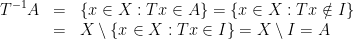
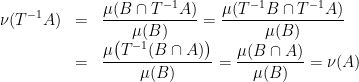
Example 3 hints that in order to find all the ergodic measures of a given system, one should look at the invariant sets (observe, however, that not all ${T}$ -invariant sets give an ergodic measure: the set ${A:=\left\{(n\pi,\pi):n\in{\mathbb Z}\right\}\subset{\mathbb T}^2}$ is invariant for the system of Example 3 and yet no ergodic measure has ${A}$ as its support).

Proposition 4 Let ${(X,{\cal B},\mu,T)}$ be a probability preserving system and let

$\displaystyle {\cal I}:=\{B\in{\cal B}:T^{-1}B=B\}$

Then ${{\cal I}}$ is a ${\sigma}$ -algebra.

Proof: Let ${I\in{\cal I}}$ and let ${A=X\setminus I}$ . Then

$\displaystyle \begin{array}{rcl} \displaystyle T^{-1}A &=&\displaystyle \{x\in X:Tx\in A\}=\{x\in X:Tx\notin I\} \\&=&\displaystyle X\setminus\{x\in X:Tx\in I\}=X\setminus I=A \end{array}$

and hence ${{\cal I}}$ is closed under complements. Now let ${(I_n)_{n=1}^\infty}$ be a sequence of sets in ${{\cal I}}$ and let ${I=\bigcup I_n}$ . Then

$\displaystyle \begin{array}{rcl} \displaystyle T^{-1}I &=&\displaystyle \{x\in X:Tx\in I\}=\left\{x\in X:Tx\in\bigcup_{n=1}^\infty I_n\right\} \\&=&\displaystyle \bigcup_{n=1}^\infty \left\{x\in X:Tx\in I_n\right\}=\bigcup_{n=1}^\infty T^{-1}I_n=\bigcup_{n=1}^\infty I_n=I \end{array}$

and hence ${{\cal I}}$ is closed under countable unions and therefore it is a ${\sigma}$ -algebra. $\Box$

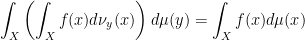
Henceforth we will call ${{\cal I}}$ the ${\sigma}$ -algebra of invariant sets. It turns out that the ergodic measures that appear in Theorem 2 are the measures that arise from the disintegration of ${\mu}$ with respect to the ${\sigma}$ -algebra of invariant sets.

Lemma 5 Under the conditions of Theorem 2, let ${{\cal A}\subset{\cal B}}$ be a ${\sigma}$ -subalgebra and let ${(\nu_y)}$ be the disintegration of ${\mu}$ with respect to ${{\cal A}}$ . Then for every ${f\in C(X)}$ there exists a set of full measure set ${Y\subset X}$ such that for every ${y\in Y}$ we have

$\displaystyle \mathop{\mathbb E}[f\mid{\cal A}](x)=\mathop{\mathbb E}[f\mid{\cal A}](y)\qquad\text{for }\nu_y\text{ almost every }x$

Proof: Let ${g=\mathop{\mathbb E}[f\mid{\cal A}]}$ . For ${x,y\in X}$ and let ${g_y(x)=|g(x)-g(y)|}$ . Then ${g_y}$ is ${{\cal A}}$ -measurable and hence

$\displaystyle \int_Xg_y(x)\,\mathrm{d}\nu_y(x)=\mathop{\mathbb E}[g_y\mid{\cal A}](y)=g_y(y)=0$

for ${\mu}$ -a.e. ${y\in X}$ . $\Box$

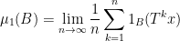
Lemma 6 For ${\mu}$ -a.e. ${y}$ , the measure ${\nu_y}$ that arises from the disintegration of a ${T}$ -invariant measure ${\mu}$ with respect to the invariant ${\sigma}$ -algebra ${{\mathcal I}}$ is ${T}$ -invariant and ergodic.

Proof: We first prove that for almost every ${y}$ , ${\nu_y}$ is ${T}$ -invariant. More precisely, we will find a set ${Y\subset X}$ with ${\mu(Y)=1}$ such that for every ${y\in Y}$ , the measure ${\nu_y}$ is ${T}$ -invariant. Let ${D\subset C(X)}$ be a countable dense set. It suffices to show that for each ${f\in D}$ there exists a set ${Y_f\subset X}$ with ${\mu(Y_f)=1}$ and such that for every ${y\in Y_f}$ we have ${\int_XTf-f\,\mathrm{d}\nu_y=0}$ . Recall by the construction of conditional measure that ${\int_XTf-f\,\mathrm{d}\nu_y=\mathop{\mathbb E}[Tf-f\mid{\mathcal I}]}$ , so we need to show that ${\mathop{\mathbb E}[Tf-f\mid{\mathcal I}]=0}$ ${\mu}$ -a.e. But this follows from the following computation, which holds for each ${I\in{\mathcal I}}$

$\displaystyle \int_ITf-f\,\mathrm{d}\mu=\int_X1_I\cdot Tf-1_I\cdot f\,\mathrm{d}\mu=\int_XT\big(1_I\cdot f\big)-1_I\cdot f\,\mathrm{d}\mu=0$

We now show that almost every ${\nu_y}$ is ergodic. It suffices to show that for every ${f\in D}$ , there exists a set ${Y_f\subset X}$ with ${\mu(Y_f)=1}$ and such that for every ${y\in Y_f}$ ,

$\displaystyle \lim_{N\rightarrow\infty}\frac1N\sum_{n=1}^NT^nf(x)=\int_Xf\,\mathrm{d}\nu_y \qquad\text{for }\nu_y\text{ almost every }x.$

The pointwise ergodic theorem (see Theorem 2 in this post, or more precisely this stronger version) implies that the left hand side equals ${\mathop{\mathbb E}[f\mid{\mathcal I}](x)}$ for every ${x}$ in a full ${\mu}$ -measure set. On the other hand, the left hand side is ${\mathop{\mathbb E}[f\mid{\mathcal I}](y)}$ (where the conditional expectations are both taken with respect to the measure ${\mu}$ ). The desired conclusion now follows from Lemma 5. $\Box$

Proof: } Let ${{\cal I}}$ denote the invariant ${\sigma}$ -algebra and let ${(\nu_y)_{y\in Y}}$ be the disintegration of ${\mu}$ with respect to ${{\cal I}}$ , for some ${Y\in{\cal B}}$ with ${\mu(Y)=1}$ . By Lemma 6 each of the measures ${\nu_y}$ is ${T}$ -invariant and ${T}$ -ergodic. By the properties of the disintegration of measures we have that for every ${f\in L^1(X,\mu)}$ , the map ${y\mapsto\int_fd\mu}$ is ${{\cal I}}$ -measurable, and hence it is ${{\cal B}}$ -measurable and ${T}$ -invariant. Moreover, it follows from the properties of the disintegration of measures that

$\displaystyle \int_X\left(\int_Xf(x)d\nu_y(x)\right)d\mu(y)=\int_Xf(x)d\mu(x)$

and this finishes the proof. $\Box$

This entry was posted in Analysis, Classic results, Ergodic Theory, Tool and tagged Choquet theorem, disintegration of measures, ergodic decomposition. Bookmark the permalink.

22 Responses to Ergodic Decomposition

Pingback: Disintegration of measures | I Can't Believe It's Not Random!
azalk says:

11/07/2014 at 3:25 am

Is $\nu=\frac1{\mu(A)}\mu|_{\cal A}$ constant over every set in ${\cal A}$ ?

Reply
- azalk says:
  
  11/07/2014 at 3:25 am
  
  sorry couldn’t get latex code to show up properly …
- azalk says:
  
  11/07/2014 at 5:44 am
  
  Also, in the statement of the theorem, wouldn’t a measure have to be assigned to a set, and not an element y of $Y \subseteq X$ ?
- Joel Moreira says:
  
  14/07/2014 at 9:11 am
  
  The measure $\nu=\left.\frac1{\mu(A)}\mu\right|_{\mathcal A}$ is not constant. Given a set $B\in{\mathcal A}$ , by definition we have $\nu(B)=\mu(B)/\mu(A)$ .
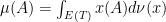
  Regarding the theorem, it assigns to each point $y\in Y$ a measure $\mu_y$ , but each of the measures $\mu_y$ is itself a function from ${\mathcal B}$ to $[0,1]$ .
mOe says:

25/02/2016 at 8:12 am

I like the present reasoning that the conditional probabilities are ergodic. I know related statements from the Maitra paper. There are proofs of this using the ergodic theorem, see e.g. the lecture notes by Omri Sarig. I always feel lost reading that proof. ( I think because the several integration variables do not appear.) Do you know that proof? Can you make it more precise? I would appreciate to understand it.

Reply
- Joel Moreira says:
  
  25/02/2016 at 5:02 pm
  
  Dear mOe, thanks for your comment!
  
  I am not familiar with Maitra’s paper. If by Omri’s notes you mean http://www.math.psu.edu/sarig/506/ErgodicNotes.pdf (it’s Theorem 2.5 there) then the proof has indeed a different flavor.
  
  The idea is to use the ergodic theorem which implies that $\displaystyle f^*:=\lim_{N\to\infty}\frac1N\sum_{n=1}^NT^nf$ is the conditional expectation of $f$ in ${\cal I}$ . In other words, $f^*(y)=\int_X f(x)d\mu_y(x)$ for almost every $y\in X$ .
  For any given $y\in X$ , if this equality holds for every $f\in C(X)$ (assuming wlog that $X$ is compact) then $\mu_y$ is indeed an ergodic measure.
  In fact it suffices to check it for a dense subset of functions, and taking a countable dense subset of $C(X)$ one obtains a full measure set of $y$ ‘s in $X$ for which $\mu_y$ is ergodic.
Ian says:

14/05/2016 at 10:35 am

I’m actually a little confused by your proof of ergodicity of the mu_y’s. Isn’t there an order of quantifiers issue here? You’re proving that for every I, you have mu_y(I)=0,1 for almost every y. But you want to show that for almost every y, you have mu_y(I) =0,1 for every I. If the sigma algebra I was countably generated, you could exchange the order, but I’m guessing that in the generic situation it is not countably generated, e.g. if T is an irrational rotation of the circle. Thoughts?

Reply
- Joel Moreira says:
  
  14/05/2016 at 12:20 pm
  
  That is indeed an interesting subtlety which I had not consider, I am afraid you are right in that one needs the $\sigma$ -algebra ${\mathcal I}$ to be countably generated which is not always the case. The simplest way I see of avoiding this issue is by removing from the whole space $X$ a set of measure $0$ (the measure is $\mu$ here) so that ${\mathcal I}$ becomes countably generated.
  That one can remove such a set follows from the classical fact that any “reasonable” measure space is isomorphic to $[0,1]$ with the Borel $\sigma$ -algebra and Lebesgue measure (for a quite nice and precise description of this theorem, see Vaughn Climenhaga’s nice posts https://vaughnclimenhaga.wordpress.com/2015/10/22/lebesgue-probability-spaces-part-i/)
- Ian says:
  
  14/05/2016 at 3:57 pm
  
  Interesting. How does it follow that you can find such a set? I don’t see how the fact that X is standard helps — I’m not sure how to do it for an irrational rotation on the circle, actually.
- Joel Moreira says:
  
  14/05/2016 at 6:49 pm
  
  Sorry, what I said did not make complete sense. What I had in mind is to identify the $\sigma$ -algebra ${\mathcal I}$ with an equivalent countably generated $\sigma$ -algebra $\tilde{\mathcal I}$ (equivalent in the sense that for any $I\in{\mathcal I}$ there exists $\tilde I\in\tilde{\mathcal I}$ such that $\mu(I\bigtriangleup\tilde I)=0$ ).
  For the case of an irrational rotation (which is already ergodic), while ${\mathcal I}$ is infinite (and actually each point $y\in X$ belongs to some set $I\in{\mathcal I}$ with $0$ measure) it is equivalent to the trivial $\sigma$ -algebra $\{\emptyset, X\}$ .
- Ian says:
  
  14/05/2016 at 7:10 pm
  
  I agree, you can prove you can’t do the other thing for the irrational rotation. I’m still a little confused, though. Don’t you still need to say at some point that for a.e. y,
  
  nu_y(I)=nu_y(tilde I) for all pairs I and tilde I as you describe?
  
  You know that the mu measure of the symmetric difference is zero, but that only tells you that the nu_y measure of the symmetric difference is zero for almost every y, which gives you the same quantifier problem, no?
  
  (Thanks for thinking about this with me. I’m trying to write down an ergodic decomposition theorem in a setting where I don’t have easy access to an ergodic theorem, so am trying to avoid it.)
- Joel Moreira says:
  
  14/05/2016 at 7:19 pm
  
  The way I’m thinking, one replaces ${\mathcal I}$ with $\tilde{\mathcal I}$ at the beginning of the argument, and take the disintegration with respect to the (countably generated) $\tilde{\mathcal I}$ , so there is no need to worry about how $I$ and $\tilde I$ differ with respect to the disintegration measures $\mu_y$ .
- Ian says:
  
  14/05/2016 at 8:34 pm
  
  Well, you still have to show that those measures are ergodic, though, which is a statement about I, not tilde I.
- Joel Moreira says:
  
  15/05/2016 at 3:53 pm
  
  You are right, the invariant sets are still the ones in ${\mathcal I}$ regardless.
  I thought a bit more about this issue, and I think it is possible to fix the proof by proving ergodicity instead by studying invariant continuous functions (the idea being that there is a countable dense subset of continuous functions), but it will take me a while to write down all the details (assuming this works at all).
Pingback: Polygonal billiards | Bahçemizi Yetiştermeliyiz
James says:

01/06/2017 at 11:17 pm

I don’t see why the final set $Y$ measurable since it is a possibly uncountable union of the $Y_\mu$. Perhaps you just meant to highlight that the measures $\nu_y$ don’t depend on $\mu$, only on $T$? In the statement of theorem 1 though, it seems that $\mu$ is just some fixed measure and in that case doesn’t it suffices to just take $Y=Y_\mu$?

Reply
- Joel Moreira says:
  
  02/06/2017 at 9:40 am
  
  You are right, one needs to pass to the completion of the Borel $\sigma$ -algebra (with respect to $\mu$ ) in order for $Y$ to be measurable. The idea is indeed that one has the ergodic measures $\mu_y$ independent of the measure $\mu$ . Of course one can obtain a weaker version of Theorem 1 where one starts with a fixed measure $\mu$ to begin with, and then one only needs the set $Y_\mu$ (which is measurable with respect to the Borel $\sigma$ -algebra). For this weaker version there is also no need for Lemma 5.
Michael says:

14/09/2017 at 11:33 am

In example 2, wouldn’t it be more proper to call the group T the circle group, and denote it S? And then X=T^2 would be the torus.

Reply
- Joel Moreira says:
  
  15/09/2017 at 1:24 pm
  
  It boils down to a choice of notation and terminology. Personally I think of $\mathbb{T}^d$ as the $d$ -dimensional torus, including for $d=1$ .
  Also I tend to use the symbol $\mathbb{T}$ for the additive group $\mathbb{R}/\mathbb{Z}$ and $S^1$ for the multiplicative group of complex numbers with absolute value 1 (of course these groups are isometrically isomorphic but it helps to distinguish additive and multiplicative notation)
Pingback: Three different entropies, variational principle and the degree formula. – Blog Tigle goes here
Pingback: Inaugural post: Three different entropies, variational principle and the degree formula. – That Can't Be Right